
The idea behind using a Markov chain process in melody creation is to speed up the compositional process by taking an existing melody and turning it into a new melody of desired length. In collaboration with Thomas Grossi, we developed a script written in Python that reads in a MIDI file, analyzes the melody’s structure, and then returns a MIDI file with a new melody of desired length based on the input file and any specified parameters (discussed below).
The plain sequence in the program follows a traditional Markov process, where it looks at the relationship between each note in the input melody and the following note. For example, in the simple eight note melody [A G G B A B G B], the computer sees that the note A goes once to G and once to B, meaning that in this melody A has a 50% chance of going to G, and a 50% chance of going to B. On the other hand, the note G is followed once by G and twice by B, meaning that G goes to G 33% of the time, and to B 66% of the time. This information is compiled into a matrix, which details the chance of any unique note in the melody transitioning to another note in the melody. The probabilities in the transition matrix are used to determine which notes will tend to follow which in the output melody. The user provides the input melody (as a MIDI file), and decides the length of the sequence.
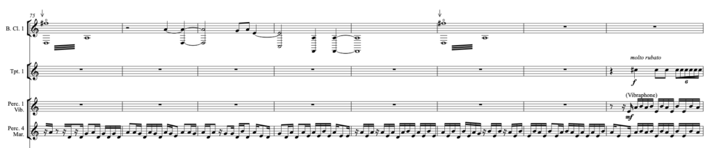
This process, as well as the following ones, were used extensively in my PhD works, but prominently featured in Sequence (below). My goal was to use the Markov sequences as one of three different layers (in combination with an electronic drone and the cello/clarinet duet above). The drone and Markov melodies provide a bed of sound, over which the other instruments are free to play a more melodic form.
Observed within the sequence is the emergence of a ‘melody rhythm’. By having a melody that is grouped with sub structures of, say, 2, 3, and 4 notes, the patterning of the resulting sequence of quavers or semi-quavers sounds complex, but is very simple in construction. What winds up happening is that one note will stand out (typically the highest or lowest note), and every time this note re-emerges the result is something that is both rhythmic as well as melodic. By playing with rhythm type and repetition in the melody before running the Markov analysis, one can end up with many different results and patterns.
On the other hand, by using a technique called mapped sequence (explained below), the melody-rhythm can shift from stable to chaotic and right back to stable again. The same concept of stability/instability applies to the harmony. There are endless possibilities.
The rest of the article below goes into specifics about how the computer code works. You can find the python code, as well as a variety of example melodies, on Thomas’s github page.
In addition to a plain sequence, four variations with diverse levels of complexity and purposes were developed, called: (a) mapped sequence, (b) sparse sequence, (c) chord sequence, and (d) grouped sequence.
The mapped sequence is a bit different, as one can build a sequence out of any number of sections, each associated with a different melody, allowing for meticulously controlled shifts between sets of notes. The sequence relies on a map file, which details several advanced parameters and can be built with the mapping toolkit module, as below:
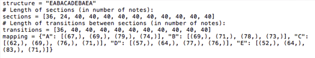
The user must provide an initial melody and any number of secondary melodies (as MIDI files), which must contain the same number of unique pitches as the initial melody (the easiest way is to provide the same melody in different keys). The mapping parameter in the map file shows the relationship between a section (identified by a letter of the alphabet) and the set of notes on which it will be based. The mandatory initial melody will always be referred to as section ‘A’. The program compiles a transition matrix for section ‘A’ and uses it to determine the relationship between all notes in the output sequence, however when building other sections, it will change the notes to their equivalent in that particular section, effectively ‘mapping’ notes from one melody onto another. For instance, following the example map, MIDI note 74 is the fourth note in the section ‘A’ set, which means it will become MIDI notes 73, 71, 76 and 71 in sections ‘B’, ‘C’, ‘D’ and ‘E’ respectively.
This technique is used extensively to modulate in the above track, Sequence. In particular, it makes use of three additional parameters of the map: the structure, the sections, and the transitions. The structure allows for an ordering of the different structures – so perhaps there is one section in C major, F major and another in G minor – you can choose the ordering of how these appear. The sections is a list of the desired lengths for each section (in the example map, the first section ‘E’ has 36 notes, next ‘A’ has 24 notes, etc.). Finally, the transitions – they are optional, but make it possible to have music (of desired length) between two sections, where the notes gradually shift from those belonging to the first section, to those belonging to the next one. In a hypothetical transition between an E section and an A section, the computer would start with a 100% probability of taking notes from the E set, and over the course of the transition have the probability of notes from A continually increase, until there is a 100% probability of taking notes from A. This causes a ‘blending’ of notes, not so dissimilar to convolving two audio files – which is perhaps why I found fusing these two techniques so interesting.
As a quick example – to modulate from keys C major to A major, it is possible to create a map based on four melodies, based on the notes in C, G, D and A major, with a structure parameter of [ABCD] and long transition lengths. This would slowly add more sharps until A major is reached. Using this modulation technique in combination with an electronic drone creates very different possibilities. For instance, one can have a drone in C major and another in A major and cross fade them, all while the sequence is modulating from C to A.
The chord sequence is a variation on the mapped sequence. As the sequence progresses, the computer has a chance of accessing the set of notes associated with the section it is building, and build chords of varied length by adding notes from the set on to those already present (up until the maximum number of notes in the set. The probability of this occurring increases as the sequence is built. This sequence can, for instance, take a chord progression of two or more notes, and make a sequence that starts with one note, and builds to the maximum number of notes in the chords. This is good for building up a repetitive section, (perhaps starting quietly and getting louder). The sequence can also be reversed, starting with many notes, and deconstructing down to one.
To use it, one starts with a single note version of the first chord in a progression. Then, a map with all the possible chords must be made. After running the program, one must use the sequence from which the single note version was taken, give the map file, and then designate how many notes increase should be applied to the sequence.
Amongst all, sparse sequence is perhaps the most different, but is also the most simple. This will take an existing sequence and, starting with one extreme of 0% or 100% and moving toward the other extreme (100% or 0% respectively) replace notes with rests (or opposite), breaking up the sequence. This is a really useful tool for introducing or winding down a sequence. It was found that replacing a note with a MIDI value of 5 (octave 0 F) was far easier than putting in a rest – this may be updated in future versions.
Grouped sequence is a lot closer to how a plain sequence works, however it separates the melody into groups of notes between rests, and treats the groups as single notes. It is these groups that are then analyzed by the Markov process. This keeps certain patterns in the output melody that would normally be lost as they encompass larger chunks than the pairs of notes normally used.